In this post, I talk about using World Models to train agents to paint with real painting software. This includes my thought process, approach, failures, and some future work in this direction I’m excited about.
If you want a quick summary, feel free to browse the original Twitter thread:
Sharing my winter break project. I tried combining @hardmaru's world models and @yaroslav_ganin's SPIRAL to see if an agent can learn to paint inside its own dream. It can! These strokes are generated purely inside a world model, yet transfer seamlessly to a real paint program. pic.twitter.com/nRfSWHQIdc
— Reiichiro Nakano (@reiinakano) January 11, 2019
Table of Contents
Introduction
Lately, I’ve been thinking about the role that constraints play in artistic style.
A few months ago, I visited the Hakone Open-Air Museum and found myself fascinated by some “paintings” that used glass shards in lieu of paint.
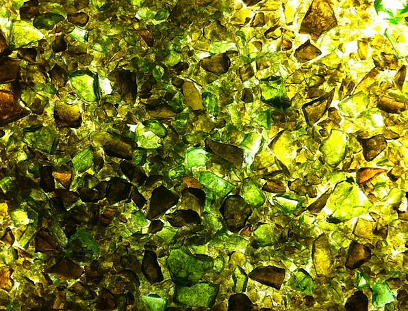
The resulting portraits were beautiful, unique, and something that could never be replicated with brushstrokes alone. All it took to achieve this new, unique style was one thing: changing the medium.
At this point, I started to think about the crucial role that the artistic medium played in creativity. It wasn’t until I saw a random Reddit post a few weeks later (on r/gaming of all places) that the idea solidified itself in my mind.
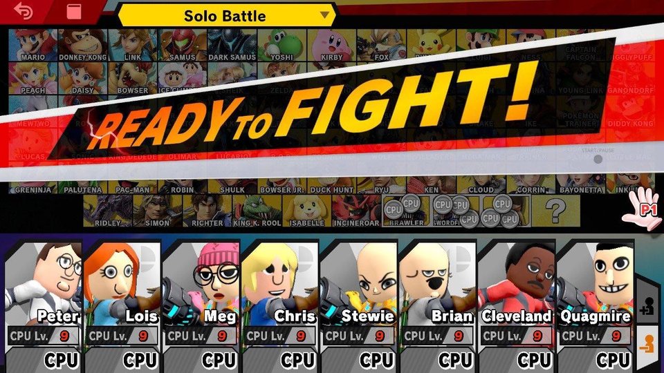
The post was quite amusing in itself. Somebody had (very painstakingly) created custom characters in Super Smash Bros. that looked like the characters from Family Guy.
However, there was a particular comment in the thread that caught my attention (and thousands of others).
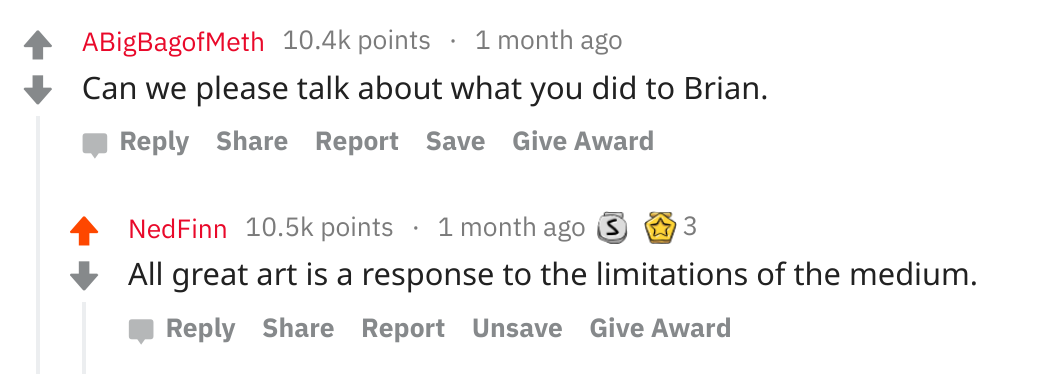
“All great art is a response to the limitations of the medium.”
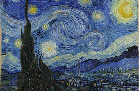
This comment summarized in the best way possible what I had been thinking of. Style can be seen as something that emerges from constraints. The Family Guy characters created above have a distinct style from the actual animated characters, simply because they were constrained to the options the game’s character creation process provides. The glass shard paintings have a distinct style from regular paintings since they were constrained to use glass shards stuck to a portrait. We can extend this idea to regular 2D portraits. Oil paintings are created with different constraints from pencil sketches. Impressionist paintings, like the famous “Starry Night”, have been constrained to use small and thin brush strokes.
This idea of constraints being beneficial to creativity turns out to be one that has been thoroughly explored. Here is an article showing some nice examples of constraints resulting in unique works of art. One of my favorites is the story of Phil Hansen, an artist who suffered a debilitating injury and ended up being unable to keep his hand from shaking. This prevented him from ever drawing again with his usual pointillist style. He eventually incorporated the squiggly lines into his artwork, resulting in his own unique style.
Today, neural networks have been used by artists, with great success, to generate 2D images that look like paintings (e.g. neural style transfer, GANs that generate portraits sold in auctions for thousands of dollars). While the results are pretty good, most of these networks are set up to directly generate each pixel of the output. This approach strikes me as odd, because artists don’t create paintings by calculating pixels one by one, they create paintings by painting.
While per-pixel calculation is in itself a constraint (in fact, I’d say the artifacts present in GAN outputs give them their own distinct style), if we wanted to have an agent replicate a piece of artwork (a painting), I imagine we’d get more realistic outputs by providing it with the same medium (a paintbrush).
It is with this mindset that I read Ha, et. al.’s work on World Models. It was not a big logical leap from here to the next step. To produce art in the way we described, an agent would need to interact with a particular constrained medium. This constrained medium could be represented by a world model.
As a proof of concept, I tried to see if an agent could learn to work with the constraints of using a paintbrush, purely by interacting with a world model of a real painting program. I chose this task as I was aware of Ganin, et. al.’s work with SPIRAL, that had indeed shown a neural network learning to work with a paintbrush. It would be a good goal to replicate their experiment results using a world model approach.
Note that the rest of this blog post assumes you have read and understood the excellent World Models article. I reuse most of the terminology from that article in this blog post.
Naively throwing the World Models code at the task
The full code for World Models is available at this repository. The first thing I did was apply the code with the bare minimum modifications to run on my task. There were two options: I could train a world model on the environment then train the agent purely on the world model (as in the Doom task), or I could train a world model but still use the outputs from the real environment during agent training (as in the CarRacing task). Since I do all my training on a single free GPU from Google Colaboratory, I opted to go for the Doom approach, as running the paint program during training would considerably slow things down. It turns out this choice would be crucial, as I would eventually need full gradients from the world model during agent training, something I would not have in the CarRacing approach.
For the paint program environment, I reused code from the SPIRAL implementation by Taehoon Kim. The implementation provides a Gym environment wrapping MyPaint and maps actions to brushstrokes and applies them to a 64x64 pixel canvas. The following table shows the environment’s action space.
| Action Parameter | Description |
|---|---|
| Pressure | Two options: 0.5 or 0.8. Determines the pressure applied to the brush. |
| Size | Two options: 0.2 or 0.7. Determines the size of the brush. |
| Jump | Binary choice 0 or 1 to determine whether or not to lift the brush for a certain stroke. |
| Color | 3D integer vector from 0-255 determining the RGB color of the brush stroke. |
| Endpoint | 2D point determining where to end the brush stroke. |
| Control point | 2D point determining the trajectory of the brush stroke. View the SPIRAL paper for more details on how the stroke trajectory is calculated. |
This action space simply mirrors that described in the SPIRAL paper. The notable exceptions are the two rather specific choices for Pressure (0.5 or 0.8) and Size (0.2 or 0.7). There is no special reason for this other than that the SPIRAL implementation I used had the environment set this way.
As a standard sanity check, my first goal was to reproduce MNIST characters with my agent. For this purpose, I disregard any Color input into the painting environment and fix everything to black.
Generating episodes
The first step is to generate episodes for training data. An episode is generated by feeding a random action to a canvas 10 times. I do this 10000 times, resulting in 10000 10-step episodes.
One thing to note is that the first action in an episode never generates a visible stroke, regardless of the value of the Jump parameter. This feature was built in to the environment I used. I assume its purpose was to allow an agent to properly select the starting position of the brush (as opposed to always starting from (0, 0)).
Training the VAE
The next step is to train the VAE on the intermediate canvas states. The VAE’s job is to compress the 64x64x3 canvas state into a single vector of length 64. To evaluate the VAE’s effectiveness in preserving the main features of the canvas, we look at the original image and its respective reconstruction.
The reconstruction seems to capture the overall shape reasonably well, but finer details are lost, especially in the later stages of an episode with multiple strokes. This result is a red flag for the approach, as it is clearly not scalable, especially as we start to deal with canvases with multiple colors and >10 strokes. A VAE simply cannot reasonably compress the domain of all multi-stroke combinations on a canvas.
Training the RNN World Model
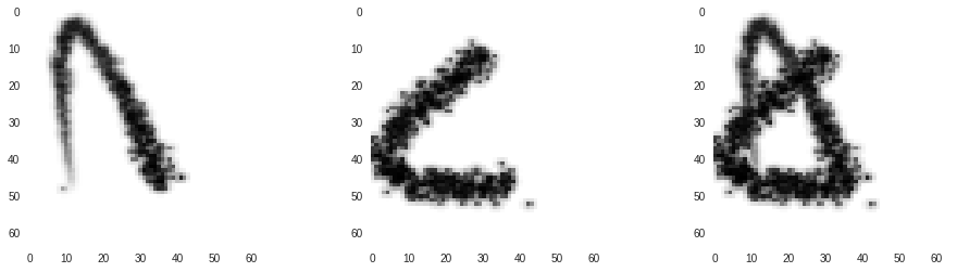
I went ahead and tried training the RNN on the 10-step episodes anyway. Given a sequence of actions, the RNN tries to predict the VAE-encoded canvas state at each step. This is then run through the VAE decoder to retrieve the actual predicted canvas.
Although the RNN learned quickly that the first action never generates a stroke, the rest of the predictions are much noisier than the target images. The approach shows promise, as the predicted images do vaguely resemble the targets, but a better method is clearly needed.
A better method: predicting individual brush strokes
The solution was simple. Instead of predicting canvases with a combination of multiple strokes, we have the world model learn only the single brush stroke produced by a particular action. This is a much smaller task for the VAE and RNN to learn.
Generating episodes
I modify the environment to clear the canvas after each step, recording only the brush stroke produced at a particular step. I also decide to increase the number of steps per episode to 20, for no particular reason other than generating more training data.


Training the VAE
The VAE does a lot better in this case, and we can see it preserve the various properties (thickness, curvature, etc.) of brush strokes very well.


Some more observations: we can see the VAE “smoothening” out the brush strokes. It also shows a bit of trouble with highly curved brush strokes that end right next to the starting point.
Training the RNN World Model
The RNN world model also predicts brush strokes a lot better. The results are slightly off when compared to the VAE reconstructions, but overall, the stroke properties still seem to be captured well.


There are two things about the RNN world model I want to note here.
First, an RNN may not actually be the optimal architecture for a world model of a painting program. Although the generated brush stroke is dependent on the previous position of the brush, we can just as easily extend the action space to take the starting position of the brush. This way, we can train a single non-recurrent network to directly map an action to an image of the brush stroke.
Second, the RNN world model has a Mixture Density Network as an output layer. This adds a non-deterministic property to the output. Although this may be useful for simulating environments with highly random behavior (Doom and CarRacing), it feels unnecessary for a world model of a relatively well-behaved paint program. Removing the MDN could result in stabler brush stroke predictions and a smaller model.
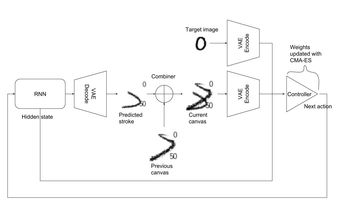
Combining brush strokes
Now that we have an RNN that can reliably predict individual brush strokes, we are missing only one more element to complete the world model of our painting program: some mechanism by which to apply successive brush strokes to a canvas. For our world model that generates only black strokes, I find a simple but effective approach to combine strokes is by choosing a pixel from either the current canvas or the new brush stroke, whichever one is darker. This is illustrated by the TensorFlow code below (assuming black is 0 and white is 255):
# Tensor containing the current state of the canvas on which to draw the stroke.
canvas = tf.placeholder(tf.float32)

# Tensor containing the brush stroke. Same shape as canvas.
stroke = tf.placeholder(tf.float32)

# mask contains a boolean Tensor with the same shape as canvas and stroke.
# mask contains True at positions where stroke > canvas (if stroke is lighter in color than canvas)
mask = tf.greater(stroke, canvas)

# out is a Tensor with the same shape as canvas and stroke
# out contains values from stroke and canvas, whichever one
# has a lower value (darker) at that point.
out = tf.where(mask, canvas, stroke)
The results of combination are shown below and compared with the actual output of the paint program.
The first row shows combination done by the actual paint program. The second row shows combination done by our combination code. Can you tell the difference?
Training the agent
The last step is to train the painting agent itself using the world model.
Following the original world models approach, my first agent was a small fully-connected neural network with a single hidden layer trained using CMA-ES. The network takes as input the RNN’s hidden state, the VAE encoded current state of the canvas, and the VAE encoded target MNIST image. It outputs 7 values, representing a full action. The architecture looked like this:
I experimented with a few different loss functions for the optimization: L2 loss between target and generated images, change in L2 loss per step (my reasoning was to reward the incremental improvement provided by each stroke), MSE between VAE-encoded target and generated images, etc. Unfortunately, this agent never learned to draw a digit. I even tried to reduce its scope by keeping only one image from the entire dataset, effectively trying to make it overfit to a single image, but this didn’t work either.
Here’s my hypothesis for why the approach failed.
I believe the agent was far too small and simple to actually learn how to paint over multiple time steps. Why then, was this agent enough to solve the Doom and CarRacing tasks? I believe it’s because in those cases, the RNN world model inherently captured information directly related to “winning” these tasks. The Doom world model learned to predict when death occurs. The CarRacing world model learned which states/actions are likely to spin a car out onto the grass. This is why, given the RNN’s hidden state, a small neural network was enough to generate an appropriate action.
On the other hand, our painter world model does not know what digits are, let alone the dynamics of drawing them. All it knows is a simple mapping from actions to brush strokes. The RNN hidden state contains far less information relating to the actual task, and thus, a more complex agent is needed to actually learn how to use the world model.
So to learn the task of drawing, I decide to make the agent much, much bigger.
I adopt the architecture of the policy network in Figure 12 of the SPIRAL paper, which was a combination of convolutional layers, MLP layers, residual blocks, and an LSTM. I tweak it a bit for my use case. The network takes as inputs the target image, the world model RNN hidden state, the previous action, and the current canvas image. Instead of an autoregressive decoder, I use a simple fully connected layer at the end that outputs the 7 values for a complete action. I did not implement the autoregressive decoder since I didn’t really understand why it was necessary, and I was quite short on time at this point (Winter break was coming to a close, and I hadn’t even cracked MNIST!).
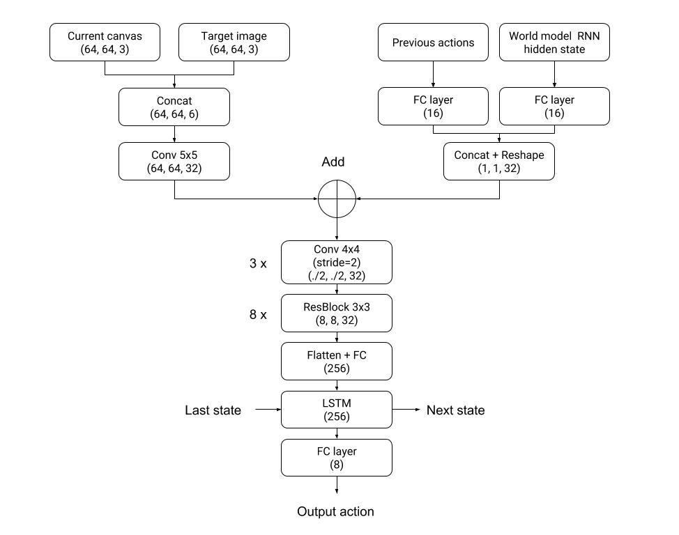
Since this agent has a lot more parameters (»10k), CMA-ES is no longer a viable optimization technique. I opt for the more standard backpropagation algorithm since the painter world model is fully differentiable and gradients from the world model output to the agent input are available. I use a WGAN-GP adversarial training procedure similar to the one used by SPIRAL to train my agent. The main difference is I could backpropagate through the painter program, so I could directly learn the agent parameters instead of using a reinforcement learning algorithm. Finally, as my goal was to reconstruct target images, I condition the network by supplying both the agent and the discriminator with the target image. The figure below shows the complete architecture.
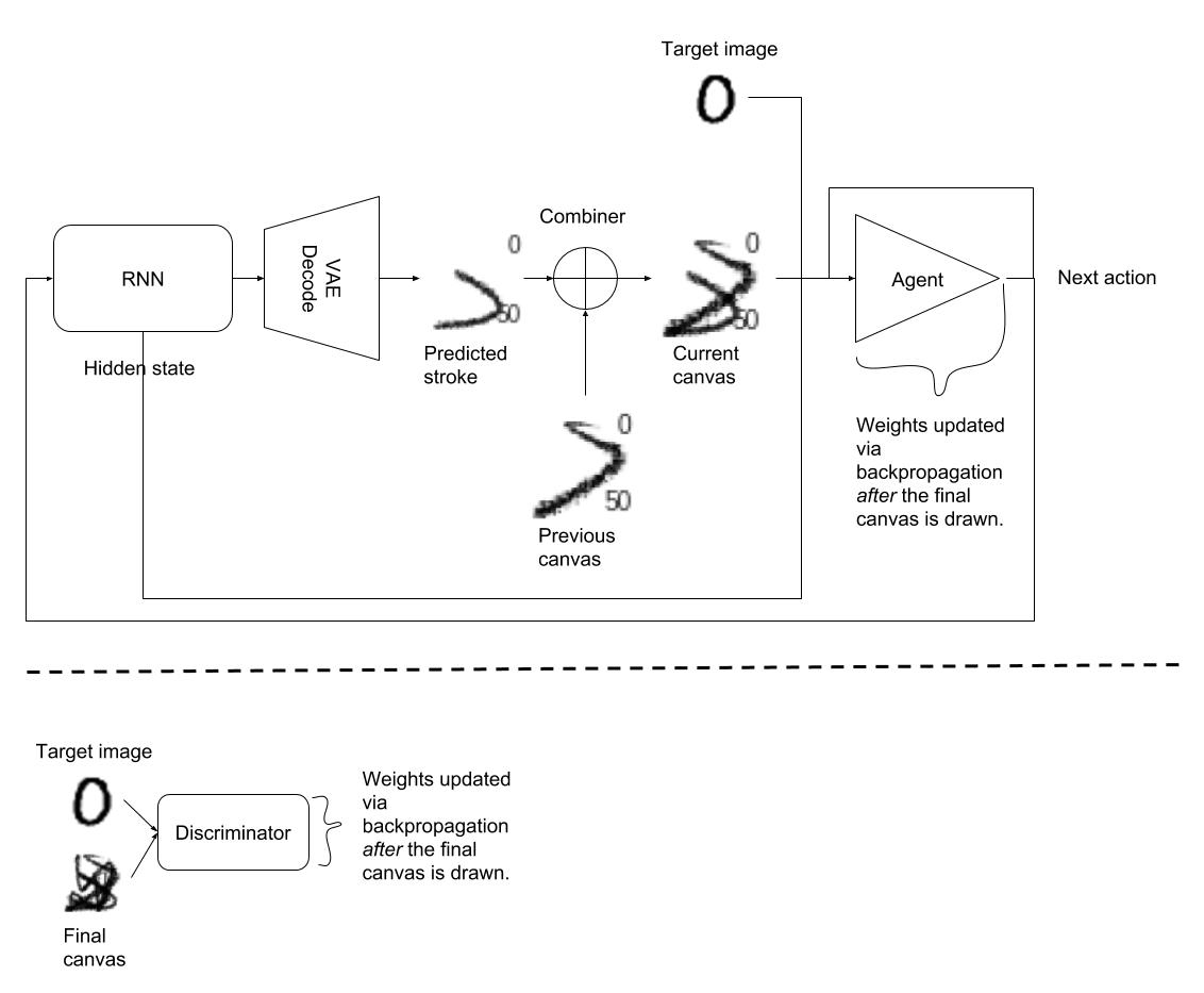
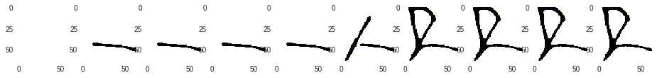
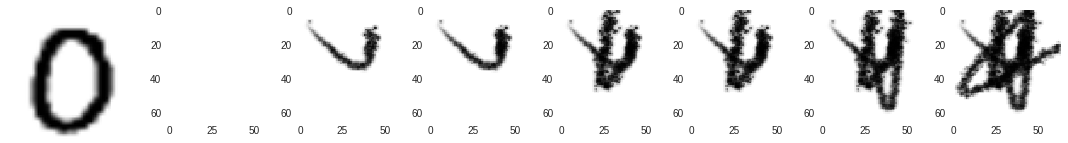
Unfortunately, when I tried training this model, it very quickly converged to not generating any strokes at all! Trying to figure out what was happening, I noticed that the Jump action parameter generated by my agent was always on, resulting in no visible strokes. Instead of trying to solve the problem, I simply sidestepped it by hardcoding the Jump parameter to 0 (I go into more depth about this behavior in the next section). This was the last missing piece, and after restarting training, my agent finally learned how to write!
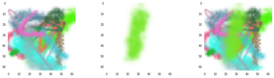
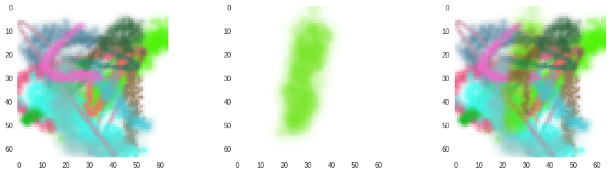
Left: Target image. Middle: World model output. Right: Generated actions transferred back to real painter environment.
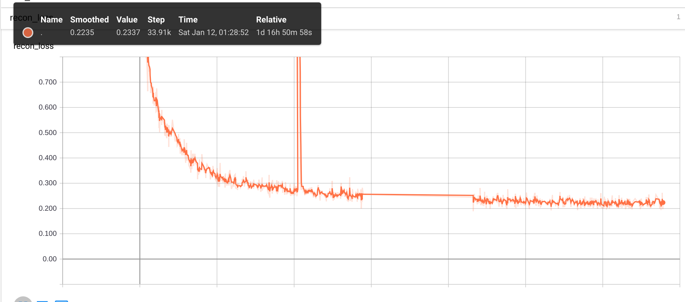
A remarkable result is how quickly the training method converges compared to SPIRAL. I show below the mean squared error between the target and generated image during training.

The graph shows the algorithm quickly reaching a mean squared error of ~0.01 (the TensorBoard value is multiplied by 10) in about ~11k steps before tapering off. I stopped things early since I was happy with the results, but it’s clear the loss was still going down. This took around 9 hours to complete on Google Colab’s free Tesla K80 GPU. In comparison, the SPIRAL agent takes on the order of 10^8 training frames, distributed among “12 training instances with each instance running 64 CPU actor jobs and 2 GPU jobs” (How much do I have to pay for this on GCP?).
On discrete actions causing imperfections in the world model
I talked about the Jump action parameter and how it killed the entire training process. To understand why this happens, we have to examine one of the main differences between a real environment and our learned world model.
A real environment can have discrete inputs and outputs, while a learned world model must learn a continuous mapping from inputs to outputs.
Our painting program environment takes only discrete actions for brush pressure (0.5 or 0.8), size (0.2 or 0.7), and jump (0 or 1). On the other hand, our world model, being a neural network, can still take values in-between, and has to dream up a smooth, continuous transition from one valid input to another. What it does in this space is up to the world model and can lead to strange results.
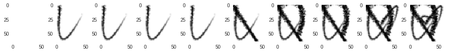
To test this, we generate a single visible (Jump = 0) stroke using the real environment. We then perform the same action on the world environment, while gradually increasing the Jump input from 0 to 1. As expected, the stroke is visible at 0 while invisible at 1, but what happens in between is interesting.
Observe how the stroke starts curving and getting fainter as we move up from 0, eventually disappearing at ~0.35. We don’t know why the world model chose this transition, but seeing as we do not give it inputs between 0 and 1 during training, we can’t really say it’s wrong either. So why does this behavior result in an untrainable agent? I attribute this to the flat region from 0.35-1 where the world model doesn’t produce any strokes. My guess is that once the agent gets into a state where it predicts any value >0.35 for Jump, the stroke becomes invisible, the gradients drop to 0, and the agent gets stuck.
We can observe the same continuous behavior to a less extreme extent for brush size and pressure (not shown).
In this case, the world model interpolates brush sizes between 0.2 and 0.7. Unlike the Jump action, the transition here is smoother, and so does not kill training with bad gradients. Unfortunately, this interpolation means the world model thinks there are brush sizes between 0.2 and 0.7, even when these do not exist in the real environment. This can result in some reconstructions looking slightly thicker or thinner when the world model actions are transferred back to the real environment.
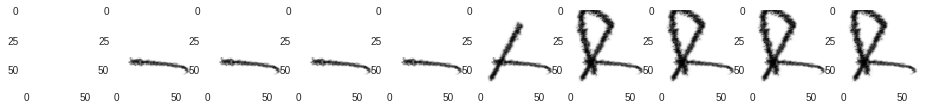
Another related consequence of using the world model instead of the real environment for training is the agent learning to exploit imperfections in the world environment. In the MNIST reconstruction task, this is evident when the agent tries to draw thick digits.
The digit being drawn here is thicker than the largest brush size the environment provides (0.7). Even in this case, our agent is somehow able to “force” the world model to output strokes thicker than 0.7 by using short, highly curved strokes. This is a glitch in the world model that does not exist in the real environment, so the actual reconstruction does not at all look like the world model’s output.
I believe that figuring out how to handle these discrete actions will be an interesting research direction moving forward. Unfortunately, we cannot always side step this issue as I have done in this case by completely ignoring the Jump action. Many interesting environments (including the MuJoCo Scenes environment solved by SPIRAL) will have unavoidable discrete actions, and if we want to apply this approach to those tasks, a better approach will be necessary.
Extending the approach to a full-color environment
Since we’ve proven the approach works on MNIST in a black and white environment, the next step is to try a full-color environment.
Also, based on the issues with discrete actions faced above, I modified the MyPaint environment to have the following action space:
| Action Parameter | Description |
|---|---|
| Pressure | |
| Size | |
| Color | 3D integer vector from 0-255 determining the RGB color of the brush stroke. |
| Endpoint | 2D point determining where to end the brush stroke. |
| Control point | 2D point determining the trajectory of the brush stroke. View the SPIRAL paper for more details on how the stroke trajectory is calculated. |
Training the VAE and RNN world model
After generating new episodes using this new modified environment, we train the VAE and RNN world model. No change in model architecture was made, aside from modifying the inputs for the new action space.
The following figure shows the results of training the brush stroke world model:


At first glance, the strokes look the same, but once you look closer, it’s obvious they’re slightly different, with the RNN predictions being a slightly worse reconstruction than the VAE outputs. Still, it is clear the world model approach works well for modeling color brush strokes.
Combining color brush strokes
Although our simplistic approach for combining brush strokes worked well for black strokes, it won’t hold up with full colors. Here’s an example of combining brush strokes using our previous method:
Instead of properly placing the stroke on top of the canvas, the algorithm just chooses the darker of both colors.
After searching for a good way to do this full-color brush stroke combination, I discovered it was actually a very common problem in computer graphics called color blending. In fact, it has been extensively discussed in the MyPaint forum itself.
One thing I realized too late was that it probably would have been appropriate to add an extra alpha channel to the 3-channel images the world model outputs, for the purpose of color blending. The MyPaint software does output an alpha channel but I discarded it prior to training the world model for simplicity.
We don’t want the new brush stroke to completely cover up what already exists. We need a way to calculate how much of the current canvas “shows through” the new brush stroke. This function is something that would have been enabled by an alpha channel. Instead of this, we just calculate the “opacity” of an individual brush stroke pixel by computing how dark it is relative to the darkest pixel (full opacity) in the brush stroke. We can then use this value as a ratio for blending the stroke with the existing paint on the canvas.
Here is some TensorFlow code illustrating this:
# A pixel ranges from 0 to 1, with [1, 1, 1] being white and [0, 0, 0] being black.
canvas = tf.placeholder(tf.float32, [-1, 64, 64, 3])
stroke = tf.placeholder(tf.float32, [-1, 64, 64, 3])

# RGB paint color chosen.
brush_color = tf.placeholder(tf.float32, [-1, 3])

# Get the "darkness" of each individual pixel in a stroke by averaging.
darkness_mask = tf.reduce_mean(stroke, axis=3)
# Make the value of a darker stroke higher.
darkness_mask = 1 - tf.reshape(darkness_mask, [-1, 64, 64, 1])
# Scale this darkness mask from 0 to 1.
darkness_mask = darkness_mask / tf.reduce_max(darkness_mask)

# Replace the original stroke with one that has all colored pixels set to the
# actual color used.
stroke_whitespace = tf.equal(stroke, 1.)
brush_color = tf.reshape(brush_color, [-1, 1, 1, 3])
brush_color = tf.tile(brush_color, [1, 64, 64, 1])
maxed_stroke = tf.where(stroke_whitespace, stroke, brush_color)

# Linearly blend
blended = (darkness_mask)*maxed_stroke + (1-darkness_mask)*canvas
The following shows the result of blending:

Agents trained with the full-color world model
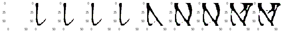
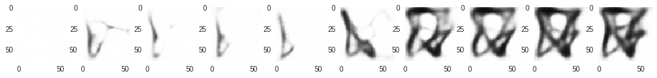
To test out the full-color world model, I trained it on two datasets: KMNIST and CelebA. Although KMNIST is a black and white drop-in replacement for MNIST, I still wanted to try it because it was a much harder and more interesting dataset than MNIST, and I thought it would be fun to tackle a new dataset that, as far as I know, hasn’t been tried using SPIRAL.
No change has been made to the adversarial training process, except the number of strokes the agent produces, which I increased from 8 to 15.
I reach an MSE of 0.018 after ~27k training steps.
The dataset is clearly more difficult than MNIST, with reconstructions being visibly noisier. Also note the highly unnatural stroke order. Still, I’d consider this a successful experiment. An interesting research direction would be to find a way to bias the model to follow natural stroke order.
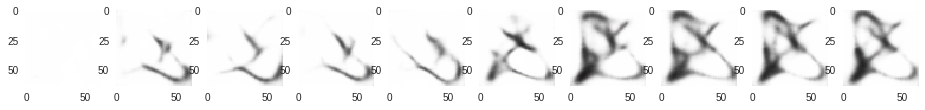
Finally, I try my first full-color dataset, CelebA. I train a 15-stroke agent and reach 0.019 MSE after ~27k steps. (Unfortunately, I wasn’t able to save my TensorBoard log files for this run…)
The results seem to be on par with the results presented in the SPIRAL paper. You can see high-level features like the hair, shirt, and background color being painted. One advantage I see is that unlike SPIRAL, my agent does not seem to make wasteful strokes that are completely covered up by later strokes. I attribute this to the ease of credit assignment when full gradients from the target image to the output image are available.
Another thing I discovered is that the reconstructions generally improve with the number of strokes the agent is allowed to use. I retrained the agent on CelebA with 30 strokes for ~26k steps, reaching an MSE of ~0.015.
The results are a lot better than the 15-stroke agent. The agent learned how to capture the shadows of faces, and decided on an interesting representation of eyes, a horizontal line across the face.
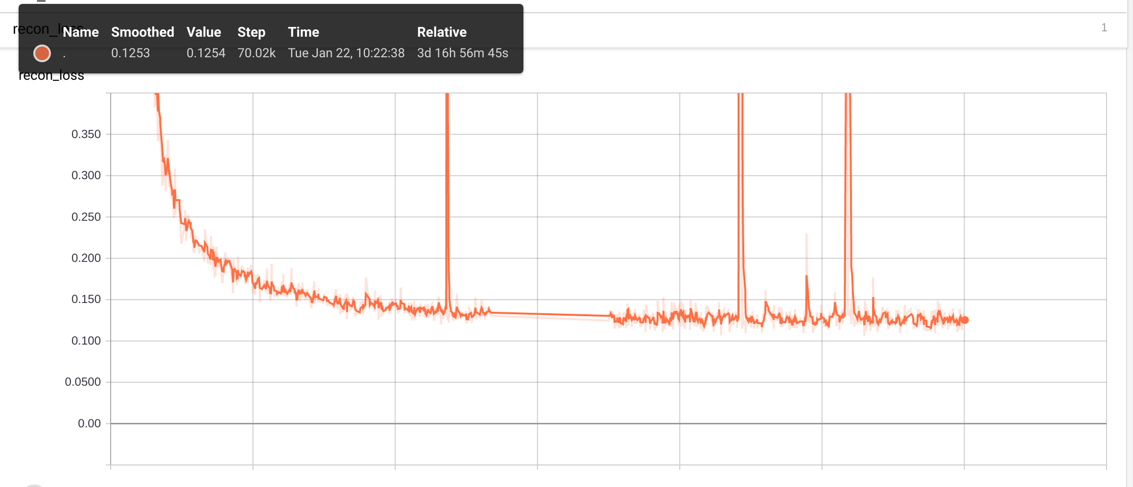
Finally, I trained a 50-stroke agent for 30k steps, reaching an MSE of ~0.0125.
The results are again better than the 30-stroke agent’s, and although the representation of eyes did not change, the agent now seems to accurately capture the jawline on most of the faces.
One thing I’m curious about is whether or not the approach will continue to scale by simply increasing the number of strokes. One thing I experienced during training the 50-stroke agent was that the training would inexplicably “collapse” from time to time and revert back to the performance of an untrained agent. I had to keep fixing it by rolling back to a previous checkpoint and resuming training. As of now, it’s unclear whether or not this is a fundamental shortcoming of the current method that will prevent it from scaling up beyond a certain amount of strokes.
Conclusion and future work
I’m personally very excited about exploring the possibilities of world models for creative ML in general. Some ideas:
- Style transfer has always been my favorite algorithm, but as mentioned in the introduction, most methods generate the outputs pixel by pixel. Painters paint by painting. Can we teach a neural network to use an actual paint brush in the style of an artist? Will the outputs be more realistic?
- Use the world model as a differentiable image parameterization. If an image classifier were given a paint brush and asked to paint a picture of the optimal dog, what would that look like? What about the optimal cat?
- Something I mentioned earlier is biasing the model for KMNIST reconstruction in some way that produces natural stroke order. If we can do this successfully, we can extract stroke data for new characters that can be used to train models like Sketch-RNN.
- Modify the constraints of the environment itself as a way to produce art. If we modified the actions to let us splatter paint on a canvas instead of using brush strokes, can we imitate Jackson Pollock’s style? Going further, we can move beyond 2D paintings. What other interesting art mediums can we learn a world model for?
If anybody has ideas for collaboration or wants to tackle some of these problems together, feel free to drop me a message. I like building awesome things with awesome people.
Acknowledgments
Here is a list of all the tools and resources I found useful while building this project. (I may have unintentionally missed some):
- World Models and the open-source world models code.
- SPIRAL
- MyPaint
- TensorFlow implementation of SPIRAL
- TensorFlow implementation of WGAN-GP
- Google Colaboratory
- WGAN and WGAN-GP
- This awesome explanation of WGAN and WGAN-GP.
- This awesome explanation of MDNs.
- Conditional GANs